Finite Element Inspired Neural PDE Solvers

Neural PDEs are a termed used to describe machine learning models which model Partial Differential Equations. Within Neural PDEs there are two different approaches; data-driven, and data-free. Data-driven approaches are similar to traditional machine learning tasks, using massive amounts of data to train highly parameterized regression models, a few examples are [LKA+21], [RMR+23] and [WWP21]. Data-free approaches, such as Physics-Informed Neural Networks [RPK19] or Neural Finite Element Networks (NFENs) [KBJ+24], [KHB+24], the work outlined in this post, do not require any ground truth data. A few other examples of data-free methods include, [LLF98], [EY17] and [SS18]. These models are optimized to minimize an objective function formulated by the target Partial Differential Equation (PDE).

Let’s use the Poisson Equation as an example.

\[\begin{split}\begin{align} - \mathbf{{\nabla}}\cdot [\nu(\mathbf{x}; q) \mathbf{{\nabla}}u(\mathbf{x}; q)] &= f(\mathbf{x}) \ \ \text{in} \ \ \Omega, \\ \alpha u + {\beta} (\nabla u\cdot \hat{\mathbf{x}{n}}) &= g(\mathbf{x}) \ \ \text{on}\ \ \Gamma_o, \end{align}\end{split}\]

Where \(u(x)\) is a scalar function indicative of the mass density, electric potential, temperature, or surface indicator function, depending on your application of the Poisson Equation. \(\nu\) is the diffusivity coefficient, and functions \(f(\mathbf{x})\) and \(g(\mathbf{x})\) are forcing functions. Lastly, different boundary conditions (Dirichlet, Neumann, Robin) are produced by varying \({\alpha}\) and \({\beta}\), e.g., \((\alpha, \beta) = (1,0)\) denotes Dirichlet boundary condition, whereas \((\alpha, \beta) = (0,1)\) represents Neumann condition.

Data-Driven Approach

In the data-driven approach to modeling the Poisson Equation one would need a dataset of field solutions for the Poisson Equation. Variability in the dataset could be from a range of diffusivity values, different boundaries conditions, etc. The machine learning model would be trained to regress the final field solution given certain input values such as diffusivity values or boundary conditions. The loss function in this scenario is most likely a simple reconstruction loss using the mean-squared-error between the predicted field solution and the ground truth field solution from the dataset.

Data-Free Approach

In the data-free approach to modeling the Poisson Equation there is no need for a dataset of ground truth values since we are constructing our loss function from the Poisson Equation itself. Constructing the data-free loss function for the Poisson Equation is very straight forward. Our neural network will make predictions of the field solution, so it will be a parameterized approximation of \(u(\mathbf{x})\). Concretely, we replace \(u(\mathbf{x})\) in the Poisson Equation with \(u_{\theta}(\mathbf{x})\) where \(u_{\theta}(\mathbf{x})\) is the predicted field solution from the neural network parameterized by \(\theta\). Since we have replaced \(u(\mathbf{x})\) with \(u_{\theta}(\mathbf{x})\), to satisfy the Poisson Equation and structure our loss function we need to find the spatial derivatives of \(u_{\theta}(\mathbf{x})\). Once we are able to compute the Laplacian of our predicted field solution \(u_{\theta}(\mathbf{x})\), we can optimize the parameters of the neural network such that its output field solution satisfies the given forcing function \(f(\mathbf{x})\).

So, by substituting our neural network, \(u_{\theta}(\mathbf{x})\), into the Poisson equation for our scalar function \(u(x)\) we get the following.

\[\begin{split}\begin{align} - \mathbf{{\nabla}}\cdot [\nu(\mathbf{x}; q) \mathbf{{\nabla}}u_{\theta}(\mathbf{x}; q)] &= f(\mathbf{x}) \ \ \text{in} \ \ \Omega, \\ \alpha u_{\theta} + {\beta} (\nabla u_{\theta}\cdot \hat{\mathbf{x}{n}}) &= g(x) \ \ \text{on}\ \ \Gamma_o, \end{align}\end{split}\]

The loss function for a data-free neural PDE Solver is given as follows.

\[\mathcal{L} = \int_{\Omega} \nu(\mathbf{x}; q)|\mathbf{{\nabla}}u_{\theta}(\mathbf{x}; q)|^2 d\mathbf{x}\]

Both methods have their trade-offs. The Data-Driven approaches have demonstrated better performance than their Data-Free counterparts at the expense of its data requirements. Data-Free methods are more aligned with the underlying PDE, but can be challenging to train and are often incapable of generalizing to unseen circumstances of the PDE it was optimized for.

Neural Finite Element Networks

The focus of this post is Neural Finite Element Networks [KBJ+24] and [KHB+24], which fall under the data-free regime and are applicable to any elliptic PDE. In data-free methods the loss function is formulated directly from the target PDE, requiring the computation of spatial gradients to formulate the target PDE. Computing these spatial gradients is not trivial, and is the major contribution of Neural Finite Element Networks. Previous methods leveraged the Automatic Differentiation framework used to optimize the parameters of the neural network to compute the spatial gradients. In Neural Finite Element Networks these spatial derivatives are computed via Finite Element Method (FEM). Computing spatial derivatives with FEM allows NFENs to directly predict a discretization of the entire field solution. If the discretization of the domain is a uniform grid, like an image, these methods are able to use any image-based neural network architecture, e.g., convolutional neural networks and vision transformers. In the following section we present NFENs through two different problem formulations our works have addressed, specifically, solving the Poisson equation over a distribution of material diffusivity coefficient fields, and solving the Poisson equation over a distribution of irregular geometries inside of the domain. We have also included a brief overview of FEM in an appendix section at the end of this post.

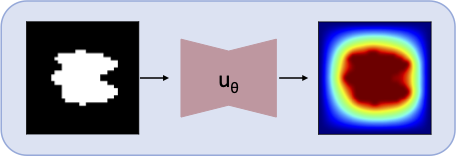
Fig. 1 Outline of an NFEN framework which maps an irregular geometry to the field solution of the given PDE, in this example the Poisson equation, to its field solution over the irregular geometry.

Neural Finite Element Networks

NFEN is a machine learning framework that learns a mapping between some input, a coefficient field, an object boundary, etc. to the field solution of the target PDE. Fig. 1 provides an overview of the NFEN framework predicting field solutions to the Poisson equation over an object boundary. The loss term for NFENs is the residual of the target PDE, where each term in the PDE is computed via FEMs. Since the entire loss term is computed from the output of the NFEN this type of model falls under the data-free regime of Neural PDE Solvers, and as our results will show, even Neural PDE Operators, capable of solving the target PDE over variable inputs not contained in the training dataset, note this is a training dataset of inputs, not ground truth field solutions.

In the following sections we cover two different applications of NFENs, where each application is a different form of input variability. The first section highlights our work in which covers variability in material diffusivity, where we show a heat or mass transfer problem through an inhomogenous media. The second section covers our work , where we implement with NFEN framework with masks of complex geometries immersed in the domain. In each section we describe the loss function formulation, and present results in 2D and 3D for the given problem formulation.

Material Properties

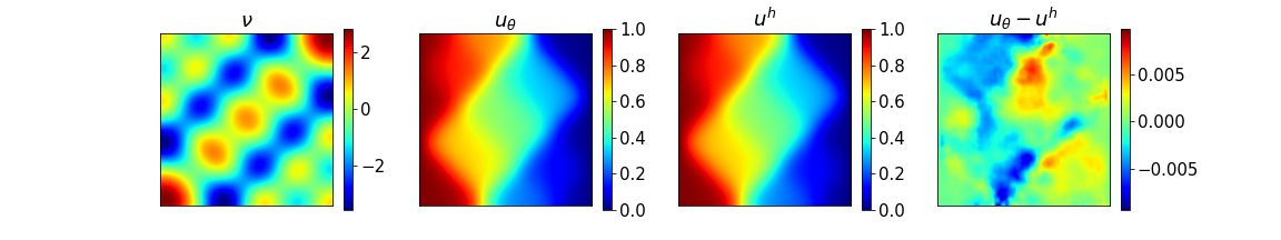
Fig. 2 Left: contours of \(ln(ν)\), the input diffusivity field; middle-left: NFEN prediction (\(u_θ\)); middle-right: reference numerical solution using FEM (\(u^h\)); right: contours of (\(u_θ - u^h\)).

For our first example problem we apply NFENs to the heat or mass transfer problem through an inhomogenous media. In this problem we created a dataset where each sample is a unique coefficient field defining the diffusivity. The NFEN learns a mapping between a distribution of diffusivity coefficient fields to the corresponding field solution of the Poisson equation. The dataset created contains \(N\) different diffusivity fields. This dataset does not contain any ground truth field solutions for the corresponding diffusivity field. The ground truth field solutions are not required to train the NFEN since the residual is computed via FEM. The loss function for this NFEN formulation is:

\[\begin{aligned} \mathcal{L} = \frac{1}{N} \sum_{i = 1}^{N} \int_{\Omega} \nu_i(\mathbf{x})|\mathbf{{\nabla}}u_{\theta}(\mathbf{x}; q_i)|^2 d\mathbf{x}, \end{aligned}\]

where \(q_i\) is our variable input, in this case the diffusivity coefficients, for NFEN, i.e., \(\nu_i\). In this problem both Dirichlet and Neumann boundary conditions are present. The Dirichlet conditions are applied exactly. The zero-Neumann condition is also applied exactly at the continuous level since the boundary integrals vanish at the continuous level.

The parameters of NFEN are optimized via gradient descent to minimize this residual across the distribution of diffusivity coefficient fields contained in the training dataset. In our works we use the Adam optimizer [KB17], but any stochastic gradient descent method can be used with minor performance differences.

Once the NFEN is trained it can approximate field solutions to unseen diffusivity fields, given they are drawn from the same distribution used to create the training dataset. This generalization ability from NFEN classifies it as a data-free Neural Operator, something in the current landscape that has not been achieved.

In Fig. 2 and Fig. 3, we present results for NFEN in two and three dimensional domains.

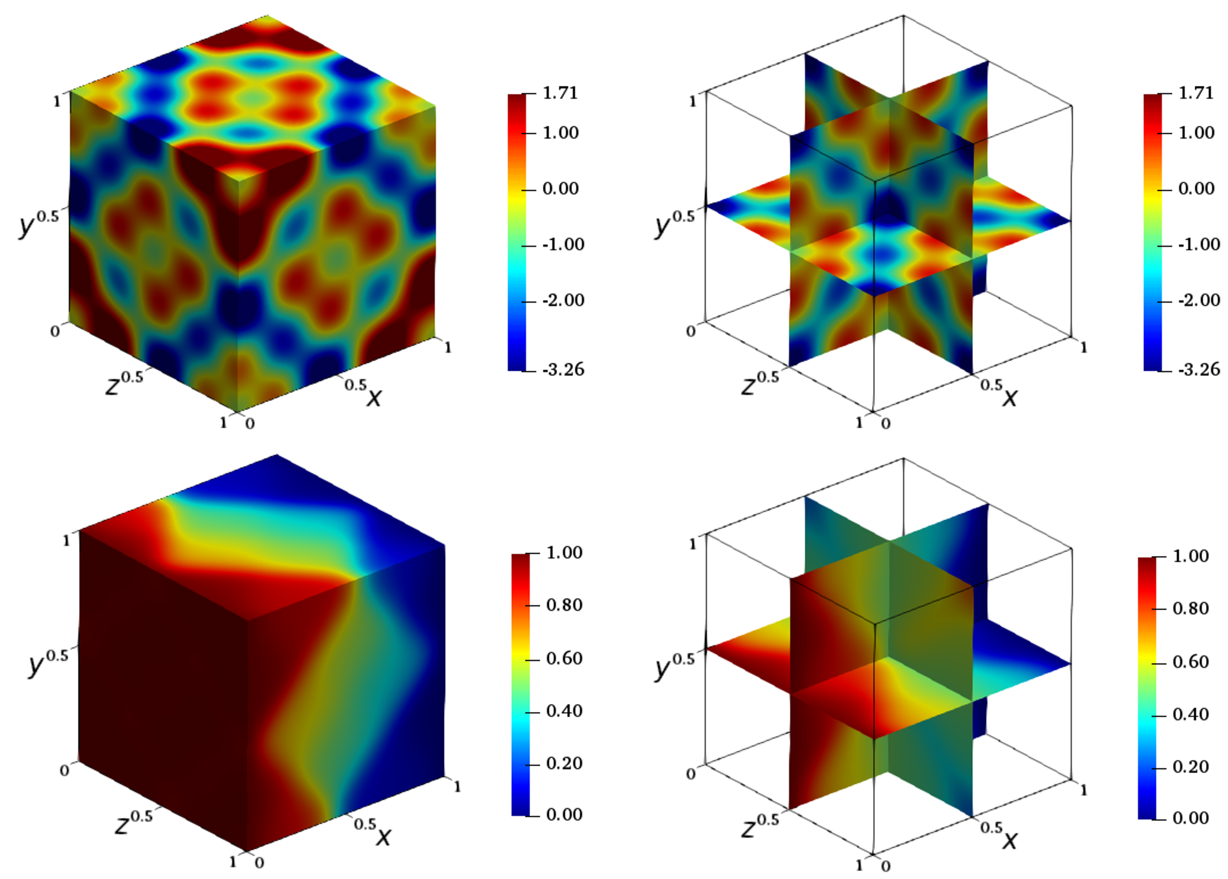
Fig. 3 Contours of \(\ln(\nu(x,y,z))\) and the solution \(u_{\theta}(x,y,z)\) to the 3D Poisson’s problem on a \( 64\times 64\times 64 \) mesh (for \( \mathbf{a} = (-1,1.4,1.5,-1.3,-1.6,0.3) \)).

Immersed Object

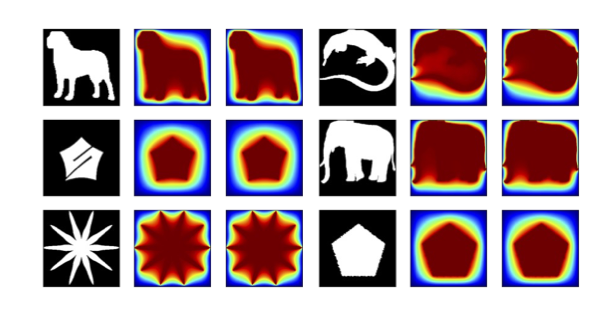
Fig. 4 Results for a single 2D NFEN which maps an unseen irregular geometry to the field solution of the Poisson equation. The first and fourth columns are the masks of the irregular geometry, the second and fifth columns are the predicted field solution, the third and sixth columns are the ground truth FEM field solution.

NFENs are very flexible and are even capable of learning field solutions of domains that contain irregular geometries such as Fig. 4. For this problem NFEN learns a mapping between a mask of the irregular geometry in the domain and the field solution which satisfies the given PDE over the domain with the irregular geometry.

Lets continue with the same Poisson equation example, but with the added boundary conditions for the irregular object. We now have,

\[\begin{split}\begin{align} - \mathbf{{\nabla}}\cdot [\nu(\mathbf{x}; q) \mathbf{{\nabla}}u_{\theta}(\mathbf{x}; q)] &= f(\mathbf{x}) \ \ \text{in} \ \ \Omega, \\ u_{\theta}(\mathbf{x},q) &= 0, \ \text{on}\ \Gamma_B, \\ \alpha u_{\theta} + {\beta} (\nabla u_{\theta}\cdot \hat{\mathbf{x}{n}}) &= g(x) \ \ \text{on}\ \ \Gamma_o, \end{align}\end{split}\]

where, in this formulation, \(q\) denotes the mask of the irregular geometry. We also have the added boundary condition which states the field solution is \(0\) on the irregular geometry.

When formulating the loss for this problem we need to pay special attention to how we compute the residual such that it respects the boundary conditions. In the Irregular Boundary Network work , we chose to strongly apply the Dirichlet boundary conditions over a discrete approximation of the irregular object. This discrete approximation of the irregular object is the binary mask of the irregular object itself, the input to the NFEN in this problem. Strongly applying the Dirichlet boundary conditions of the irregular object amounts to applying a threshold function over the predicted field solution by the Irregular Boundary Network. Once boundary conditions have been applied the field solution, with applied boundary conditions, is passed off to the FEM-based loss function to compute the residual as is done in the previous NFEN example.

The training dataset for this problem is a distribution of irregular geometries, opposed to diffusivity fields in the previous problem. The distribution of these ’irregular geometries’ may vary wildly, as the binary images in Fig. 4 show. The results shown in Fig. 4 come from a similar distribution as the training dataset, but are all samples from the test dataset.

The loss function for this problem is as follows,

\[\begin{aligned} \mathcal{L} = \frac{1}{N} \sum_{i = 1}^{N} \int_{\Omega} |\mathbf{{\nabla}}u_{\theta}(\mathbf{x}; q_i)|^2 d\mathbf{x}, \end{aligned}\]

where \(N\) is a mini-batch of irregular geometries from the training dataset and \(q_i\) is a single irregular geometry in the minibatch.

As with the previous example problem the parameters of the NFEN are optimized with the Adam optimization algorithm and a standard UNet architecture. Once optimized the NFEN can reliably predict field solutions to irregular boundaries not contained in the training dataset. This second example supports the potential for neural networks to learn PDEs in a data-free regime without the need to be retrained for a new unseen input geometry.

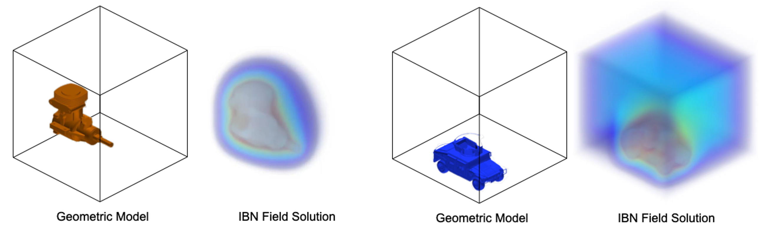
Fig. 5 Geometric model with the domain (left) and the field solution to Poisson’s equation using the NFEN framework (right) for the Engine and the Humvee models.

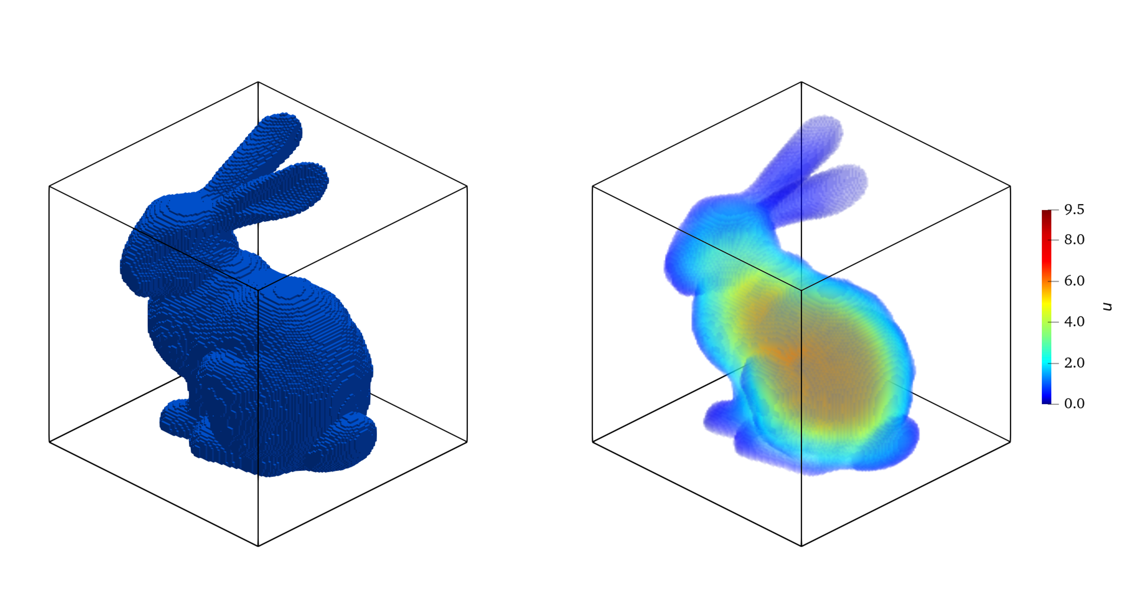
Fig. 6 Left: the “Stanford bunny” placed within the background domain; Right: a single-instance NFEN for the Poisson equation is solved on the bunny using NFEN. The forcing \(f = 500\), and the boundary condition is given by \(u = 0\) on the surface of the bunny. This is an example where the solution is sought inside the object rather than outside.

Conclusion

Overall Neural Finite Element Networks provide a clean and simple framework to learn Neural PDE Solvers and potentially Operators without the need for any expensive ground truth field solutions.

• Provides a flexible framework for any elliptic PDE.

• Approximates a discretized field solution.

• Is agnostic to the network input, i.e., diffusivity coefficient fields, immersed irregular geometries, etc.

• Can be used with any network architecture, Convolutional Neural Networks, Vision Transformers, and even Graph Neural Networks.

• Builds off of decades of work dedicated to numerical methods.

For more information on Neural Finite Element Networks, please see our works [KBJ+24] and [KHB+24].

References

[EY17]

Weinan E and Bing Yu. The deep ritz method: a deep learning-based numerical algorithm for solving variational problems. 2017. arXiv:1710.00211.

[KBJ+24] (1,2,3)

B. Khara, A. Balu, A. Joshi, and others. Neufenet: neural finite element solutions with theoretical bounds for parametric pdes. Engineering with Computers, 2024. doi:10.1007/s00366-024-01955-7.

[KHB+24] (1,2,3)

Biswajit Khara, Ethan Herron, Aditya Balu, Dhruv Gamdha, Chih-Hsuan Yang, Kumar Saurabh, Anushrut Jignasu, Zhanhong Jiang, Soumik Sarkar, Chinmay Hegde, Baskar Ganapathysubramanian, and Adarsh Krishnamurthy. Neural pde solvers for irregular domains. Computer-Aided Design, 2024. doi:https://doi.org/10.1016/j.cad.2024.103709.

[KB17]

Diederik P. Kingma and Jimmy Ba. Adam: a method for stochastic optimization. 2017. arXiv:1412.6980.

[LLF98]

I.E. Lagaris, A. Likas, and D.I. Fotiadis. Artificial neural networks for solving ordinary and partial differential equations. IEEE Transactions on Neural Networks, 1998. doi:10.1109/72.712178.

[LKA+21]

Zongyi Li, Nikola Kovachki, Kamyar Azizzadenesheli, Burigede Liu, Kaushik Bhattacharya, Andrew Stuart, and Anima Anandkumar. Fourier neural operator for parametric partial differential equations. 2021. arXiv:2010.08895.

[RPK19]

M. Raissi, P. Perdikaris, and G.E. Karniadakis. Physics-informed neural networks: a deep learning framework for solving forward and inverse problems involving nonlinear partial differential equations. Journal of Computational Physics, 2019. doi:https://doi.org/10.1016/j.jcp.2018.10.045.

[RMR+23]

Bogdan Raonić, Roberto Molinaro, Tim De Ryck, Tobias Rohner, Francesca Bartolucci, Rima Alaifari, Siddhartha Mishra, and Emmanuel de Bézenac. Convolutional neural operators for robust and accurate learning of pdes. 2023. arXiv:2302.01178.

[SS18]

Justin Sirignano and Konstantinos Spiliopoulos. Dgm: a deep learning algorithm for solving partial differential equations. Journal of Computational Physics, 2018. doi:https://doi.org/10.1016/j.jcp.2018.08.029.

[WWP21]

Sifan Wang, Hanwen Wang, and Paris Perdikaris. Learning the solution operator of parametric partial differential equations with physics-informed DeepONets. Science Advances, 2021. doi:10.1126/sciadv.abi8605.

Finite Element Methods

Finite element methods (FEM) are a class of general numerical methods used to solve PDEs by discretizing the solution space into smaller components, called ’elements’. Each of these elements is representative of a smaller and much simpler equation than the PDE governing the given domain. One can solve this larger, more complex PDE by solving the system of smaller element-wise equations.

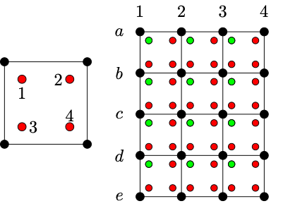
Fig. 7 Left: A single 2D element in FEM, with black dots denoting “nodes” and red dots denoting 2×2 Gauss quadrature points. Right: A finite element mesh, with 4×3 linear elements and 5×4 nodes. Each of these elements contains Gauss points for integration to be performed within that element. Within each element, the “first” quadrature point (marked “1” on left) is marked green, and others red.

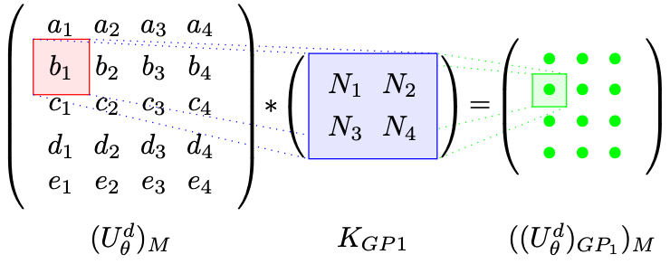
Fig. 8 Quadrature quantity evaluation in FEM context. \((U_θ^d)_M\) is the matrix view of the nodal values. \(K_{GP1}\) is kernel containing the basis function values at “gauss point - 1” (top left corner). This convolution results in the function values evaluated at the Gauss point “1” of each element (marked green). \(((U_θ^d)_{GP1})_M\) is the matrix of this result. Function values (or their derivatives) evaluated at Gauss points can then be used in any integral evaluation. For example, \(\int u^h dD = |J| \sum_{I\in M} \left[\sum_{i=1}^{4}(w_i (U^d_θ)_{GPi})_M\right]\), where \(|J|\) is the transformation Jacobian for integration and \(w\) are the quadrature weights.

Discretization: Elements and Basis Functions

Most often the domain is defined by a mesh. For simplicity, we’ll assume our domain is a uniform grid in 2D, simply an image. The nodes defining our domain are the pixels in the image. The elements used in the FEM computations will be the area between neighborhoods of adjacent nodes. Fig. 7 provides a visual of constructing a single element. In this example an element can also be thought of as the resulting pixel from a 2D convolution operation with a kernel size of \((2,2)\) and a stride of \(1\). The values of each element is defined by an interpolation operation between each node in the neighborhood. These interpolation functions, also known as basis functions, are non-parametric, and are defined a priori. These basis functions form the most critical part of the approximation of the solution function in the spatial domain. The choice of basis function is depenedent on the PDE being solved for. Linear bases are used most commonly because of their simpler implementation and interpretations, but higher-order bases are often used to obtain better accuracy.

Using FEM to Compute Spatial Derivatives of Field Solutions

Going back to our example of the Poisson Equation, to solve for the field solution \(u(x)\), where \(u(x)\) is a uniform 2D grid, we need to compute the spatial derivatives since \(\nabla u(\mathbf{x}) = u_{xx} + u_{yy}\). Computing the spatial derivatives of an image using FEM reduces to evaluating each \(2\times2\) neighborhood of pixels with the set of basis functions at the desired derivative, i.e., to compute \(u_{xx}\) we evaluate the field solution with the second derivative of the basis function for every element in the domain along the x-direction. One can also view this as a convolution operation with a \((2,2)\) kernel and stride \(1\) where we define each element in the convolution kernel to be the second derivative of the basis function. The same operation is carried out again for the 2D case, but with the derivative in the y-direction. Now that we have the \(u_{xx}\) and \(y_{yy}\) terms all we need to do is evaluate the forcing function, \(f(x)\), with our basis functions. Note, we evaluate the forcing function with the original basis functions, not the derivatives of the basis functions.

Summary

FEM are fast approximations of the spatial derivatives in a domain defined by a mesh. If the mesh is posed as a uniform 2d grid, an image, then we can seamlessly integrate FEMs into the loss function of standard vision neural networks, such as CNNs and ViT. The ability to use such network archictectures alleviates the scaling bottleneck previously imposed on data-free Neural PDE Solvers.