Submodules¶

AutoFiber generator¶

autofiber.generator.calcunitvector(vector)¶: Returns the unit vector of the given vector.

class autofiber.generator.AutoFiber(cadfile=None, initpoint=None, initdirection=None, initnormal=None, materialproperties=(228.0, 0.2, None), fiberint=0.1, angle_error=0.01, accel=False)¶

Bases: object

assign_vertices()¶

Assign all vertices a uv coordinate based on the closest geodesic to the vertex Cleanup methods are employed here such as self.fill_missing_geodesics and self.fill_low_density_geodesics

Returns: Sets the self.geoparameterization

average_fpoint(leftover_idxs, mask)¶

Last ditch effort to assign the missed vertices. Simply average any nearby uv coordinates and make sure the new coordinate won’t flip the triangle.

Parameters

leftover_idxs – Indices of missed vertices during assignment
mask – Surface vertex index mask

Returns

Any vertex indices that were missed by this cleanup method

calc_geodesic(point, element, unitfiberdirection, uv_start, direction=1, parameterization=False, save_ints=True)¶

Calculates the geodesic path from a point in a given direction

Parameters

point – The geodesic’s starting point
element – The first element we will traverse
unitfiberdirection – The desired direction the geodesic will propogate
uv_start – Starting point in uv space
direction – Positive (1) or negative (-1) direction of unitfiberdirection?
parameterization – Do we want to save this geodesic into self.georecord for use in the parameterization?
save_ints – Do we want to save intersection points for plotting purposes?

Returns

Adds the resulting geodesic path to the self.geoints and/or the self.georecord

calc_geodesics(startidx)¶: Computes the a geodesic path in the positive and negative direction for each point define in start_points beginning at the index startidx :param: startidx: Which index in self.startpoints to begin calculating geodesics at :return: Adds the relevant details for each geodesic to self.georecord

calcorientations_abaqus(modellocs, vertices, vertexids, inplanemat, texcoords2inplane, boxes, boxpolys, boxcoords)¶

Function optimized for Abaqus to determine the orientations of given locations.

Parameters

modellocs – Points of interest on the surface or close to the surface
vertices – Vertices of the model
vertexids – Indices of the vertices of the model for each element
inplanemat – Orthogonal matrix defined by spatialnde
texcoords2inplane – Transformation matrix between 3D space and uv space
boxes – spatialnde polygon box definition
boxpolys – spatialnde polygon definition relative to boxes
boxcoords – spatialnde box vertex coordinates

Returns

Orientations at modellocs

calctransform(parameterization)¶

Calculate the transformation matrix between the 3D model and the uv parameterization using spatialNDE

Parameters: parameterization – uv parameterization
Returns: Transformation matrix

check_negative_area(record)¶

Check to see if we have a triangle with a flipped normal

Parameters: record – Parameterization we want to check
Returns: True if there is a flipped triangle, False otherwise

create_parameterization()¶: Create the uv parameterization based on the computed geodesic paths If vertices can’t be assigned or are missed cleanup methods are employed to attempt to solve coordinates for all vertices. This is difficult to make robust as geometric complexities can vary quite largely.

determine_surface(initpoint, initdirection)¶

Determine which surface of a 3D model we should operate on. This should single out a solo surface without sharp (90 degree) edges

Parameters

initpoint – Starting point
initdirection – Starting direction

Returns

Sets self.surface_vertexids

fiberoptimize(seed, precision=None, maxsteps=None, lr=None, decay=None, eps=None, mu=None)¶

Minimum strain energy optimization of a seed parameterization. Uses an RMSprop optimization algorithm.

Parameters

seed – Initial uv parameterization
precision – Termination threshold for the strain energy optimization
maxsteps – Maximum number of optimization iterations
lr – Optimization rate (similar to learning rate in machine learning optimizers)
decay – Decay rate
eps – Error precision value
mu – Momentum value

Returns

fill_low_density_geodesics(minassigned)¶

Spin off more geodesics in elements that contain a low number of geodesics per area (This method is a little unreliable because the geodesics/area threshold isn’t well defined for all models)

Parameters: minassigned – Minimum number of neighbors that contain geodesics
Returns: Nothing

fill_missing_geodesics(elements, minassigned)¶

Spin off more geodesics in elements that contain no geodesics (i.e. fill holes in the initially spawned geodesics)

Parameters

elements – Elements without an geodesics
minassigned – Minimum number of neighbors that contain geodesics

Returns

Nothing

find_close_geodesic(elements, point)¶

Find the closest geodesic in self.georecord and elements

Parameters

elements – A given set of search elements for a close geodesic
point – The point we want to find a close geodesic to

Returns

tuple(georecord, element closest geodesic is in,

[vector perpendicular to u direction norm(vector) = v distance, u distance])

find_startpoints(initpoint, initdirection, normal, cfpoint, directions=(1, - 1))¶

Determines starting location, direction, and element for each geodesic Spawns geodesics perpendicular to initdirection Geodesic start points are dropped in self.fiberint intervals

Parameters

initpoint – Starting location (should be close to the center of the model)
initdirection – Starting direction vector
normal – Surface normal vector
cfpoint – initpoint location in parameterization space
directions – A tuple of positive and negative directions to compute start point geodesics

Returns

Appends new geodesic start information to the relevant lists

interpolate(leftover_idxs, mask)¶

Basic interpolation of uv coordinates based on nearby element fiber directions leftover from geodesic paths

Parameters

leftover_idxs – Indices of missed vertices during assignment
mask – Surface vertex index mask

Returns

Any vertex indices that were missed by this cleanup method

interpolate_geodesic(point, element, minassigned)¶

Determine a geodesics starting direction and uv parameterization location that is between two other geodesics

Parameters

point – A point between two geodesics
element – The element point is within or a vertex of
minassigned – Minimum number of neighbor elements that have geodesics within them for the used starting element

Returns

The direction and uv parameterization location of the geodesic at point

interpolate_point(vertex)¶

Determine the uv coordinates of a point using the same method as interpolate_geodesic (Currently not being used as direct assignment is faster and more accurate than spinning off more geodesics)

Parameters: vertex – Starting vertex
Returns: uv coordinates of vertex

layup(angle, orientation_locations=None, precision=0.0001, maxsteps=10000, lr=0.001, decay=0.7, eps=1e-08, mu=0.8, directory='out', plotting=False, save=False, model_save=None)¶

Once the parameterization has been computed we can calculate any fiber orientation without needing to compute a new geodesic mapping. Simply rotate the geoparameterization by angle and then minimize the strain energy.

Parameters

angle – Desired fiber orientation
orientation_locations – Optional locations to calculate the fiber orientations at. Default is element centroids.
precision – Termination threshold for the strain energy optimization
maxsteps – Maximum number of optimizaiton iterations
lr – Optimization rate (similar to learning rate in machine learning optimizers)
decay – Decay rate
eps – Error precision value
mu – Momentum value
plotting – Do we want to plot the results using matplotlib?
save – Do we want to save the fiber orintations at orientation_locations to a .npy file
model_save – Export an x3d model with the optimized uv coordinates defined

Returns

texcoords2inplane - Transformation matrix between 3D space and 2D space, once created any orientation

at any point on the surface can be evaluated.

loadobj()¶: Load a given CAD model using SpatialNDE Currently supported models are X3D, STL, and De-La-Mo/DMObjects

loadvars()¶: Load spatialnde data into the corresponding model variables

point_in_polygon_3d(vertices, point, inplanemat)¶: assumes vertices are coplanar, with given orthonormal 2D basis inplanemat.

AutoFiber geodesic¶

exception autofiber.geodesic.EdgeError¶: Bases: Exception

autofiber.geodesic.angle_between_vectors(v1, v2)¶: Returns the angle in radians between vectors ‘v1’ and ‘v2’ https://stackoverflow.com/questions/2827393/angles-between-two-n-dimensional-vectors-in-python

autofiber.geodesic.calcbarycentric(point, element_vertices)¶

Convert 3d point to barycenteric coordinates https://en.wikipedia.org/wiki/Barycentric_coordinate_system https://math.stackexchange.com/questions/2292895/walking-on-the-surface-of-a-triangular-mesh

Parameters

point – 3d point
element_vertices – Vertices of current element

Returns

point in barycenteric coordinates

autofiber.geodesic.calcbarycentricdirection(vector, element_vertices)¶

Convert a direction vector from 3d to barycenteric coordinates https://en.wikipedia.org/wiki/Barycentric_coordinate_system https://math.stackexchange.com/questions/2292895/walking-on-the-surface-of-a-triangular-mesh

Parameters

vector – Direction vector in 3d
element_vertices – Vertices of current element

Returns

Vector in barycenteric coordinates (du, dv)

autofiber.geodesic.calcclosestpoint(unitvector, oldpoint, meshpoints, normal)¶

Find closest mesh vertex defined by the distances calculated in calcdistance

Parameters

unitvector – Reference direction vector
oldpoint – Start point for unitvector
meshpoints – All test points

Returns

Closest point relative to unitvector

autofiber.geodesic.calcdistance(unitvector, oldvertex, meshpoints)¶

Calculate perpendicular distance between a ray and a point

Parameters

unitvector – Reference vector to calculate distance from
oldvertex – Start point for unitvector
meshpoints – Test points

Returns

Perpendicular and parallel distance to each mesh point

autofiber.geodesic.calcnormal(points)¶: Returns the normal for the given 2d points

autofiber.geodesic.calcunitvector(vector)¶: Returns the unit vector of the vector.

autofiber.geodesic.check_inplane_pnt(point, element_vertices)¶

Determines if a point is within the plane of the current element face

Parameters

point – A point within or on the edge of the current element
element_vertices – Vertices of current element

Returns

True if the point is within in the plane, or False if otherwise

autofiber.geodesic.check_inplane_vector(vector, normal)¶

Determines if a vector is in plane with the current element

Parameters

vector – Test vector
normal – Normal of element

Returns

autofiber.geodesic.check_intersection(p1, q1, p2, q2)¶: Check for an intersection between (p1, p2) and (q1, q2) https://www.geeksforgeeks.org/check-if-two-given-line-segments-intersect/

autofiber.geodesic.check_proj_inplane_pnt(point, element_vertices)¶

https://math.stackexchange.com/questions/544946/determine-if-projection-of-3d-point-onto-plane-is-within-a-triangle

Parameters

point – Test point to check
element_vertices – Vertices of current element

Returns

True or False, depending on if the projected point is inside or outside

autofiber.geodesic.find_edge(point, direction, bary, error)¶

Determines which edge number is intersected first (0, 1, 2) -> (d12, d23, d31) https://math.stackexchange.com/questions/2292895/walking-on-the-surface-of-a-triangular-mesh

Parameters

point – Start point
direction – Current fiber direction
error – Numerical tolerance

Returns

Edge number (0, 1, 2) or -1 if on an edge

autofiber.geodesic.find_element_vertex(point, unitvector, curnormal, vertices, vertexids, facetnormals)¶

Determines which element is next given a vertex and an angle

Parameters

point – Vertex in the mesh
unitvector – Fiber direction vector
curnormal – Current element normal direction vector
vertices – Mesh vertices
vertexids – Id’s of mesh element vertices
facetnormals – Normals of each element in mesh

Returns

The element in which the fiber direction vector resides

autofiber.geodesic.find_element_within(point, unitvector, normal, vertices, vertexids, facetnormals, inplanemat)¶

Determines which element a point is within

Parameters

point – Vertex in the mesh
unitvector – Fiber direction vector
normal – Current element normal direction vector

Returns

The element that the point is within

autofiber.geodesic.find_intpnt(P1, P2, P3, P4)¶: Line-Line intersection method Returns: A point in 2d that intersects line P1P2 and P3P4 https://en.wikipedia.org/wiki/Line%E2%80%93line_intersection

autofiber.geodesic.find_neighbors(element, vertexids_indices, adjacencyidx)¶

Finds neighboring elements

Parameters

element – Current element
vertexids_indices – Indices of the mesh indices
adjacencyidx – Built from spatialnde, index of element adjacency

Returns

An array of element numbers that neighbor the current element

autofiber.geodesic.invcalcbarycentric(pointuv, element_vertices)¶

Convert barycenteric coordinates into 3d https://en.wikipedia.org/wiki/Barycentric_coordinate_system https://math.stackexchange.com/questions/2292895/walking-on-the-surface-of-a-triangular-mesh

Parameters

pointuv – Point in barycenteric coordinates (u, v)
element_vertices – Vertices of current element

Returns

pointuv in 3d coordinates (x, y, z)

autofiber.geodesic.invcalcbarycentricdirection(vectoruv, element_vertices)¶

Convert vector in barycenteric coordinates into a 3d vector https://en.wikipedia.org/wiki/Barycentric_coordinate_system https://math.stackexchange.com/questions/2292895/walking-on-the-surface-of-a-triangular-mesh

Parameters

vectoruv – Vector in barycenteric coordinate (du, dv)
element_vertices – Vertices of current element

Returns

Vectoruv in 3d space (dx, dy, dz)

autofiber.geodesic.proj_vector(vector, newnormal)¶

Project a vector onto a surface defined by newnormal

Parameters

vector – Vector to be projected
newnormal – Normal of projected surface

Returns

Vector projected on surface defined by newnormal

autofiber.geodesic.rot_vector(oldnormal, newnormal, vector, terminate_angle=85.0, force=False)¶: Rotate a vector given an axis and an angle of rotation Returns: Vector reoriented from an old element face to a new element https://en.wikipedia.org/wiki/Rodrigues’_rotation_formula

autofiber.geodesic.traverse_element(af, element, point, unitfiberdirection, length, uv_start, direction=1, parameterization=True)¶

Traverse a triangular element

Parameters

af – Autofiber object
element – Current triangular element
point – Current point
unitfiberdirection – Current direction vector
length – Current length of the geodesic
uv_start – Start point of geodesic in uv space
direction –
1. for positive geodesic direction, (-1) for negative geodesic direction
parameterization – Are we going to record geodesic details for use in parameterization calculation?

Returns

next intersection point, next unitfiberdirection based on next element, next element

autofiber.geodesic.vector_inbetween(v1, v2, v3, error=1e-10)¶

Determines if a vector (v1) is between v2 and v3 https://stackoverflow.com/questions/13640931/how-to-determine-if-a-vector-is-between-two-other-vectors

Parameters

v1 – Test vector
v2 – Given vector
v3 – Given vector

Returns

True if vector is between v2 and v3, false if not between

AutoFiber optimization¶

autofiber.optimization.build_checkerboard(w, h)¶

https://stackoverflow.com/questions/2169478/how-to-make-a-checkerboard-in-numpy Build a checkerboard array

Parameters

w – width of checkerboard
h – height of checkerboard

Returns

checkerboard array of width w and height h

autofiber.optimization.calc2d(obj, points)¶

Calculate a 2D representation of a 3D model

Parameters

obj – spatialnde object
points – 3D model points to be converted to 2D

Returns

points in 2D space

autofiber.optimization.calcunitvector(vector)¶: Returns the unit vector of the vector.

autofiber.optimization.computeglobalstrain(normalized_2d, fiberpoints, vertexids, stiffness_tensor)¶

Compute the strain energy between a 2d representation of a surface and a uv (geodesic) parameterization

$p_{3D}$ - 2D mapping of 3D model surface based on element normal and inplanemat

$p_{UV}$ - Parameterization of 3D surface based on geodesic lines

Compute the areas of each triangular element in UV space:

$A_{uv} = \frac{1}{2}det(p_{uv})$

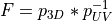
Compute the deformation gradient between each element in UV space and the corresponding element in 2D space:

$F = p_{3D} * p_{UV}^{-1}$

Utilizing the Lagrangian finite strain tensor:

$\epsilon = \frac{1}{2}(C - I)$

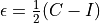
where $C = F^{t}F$ the right Cauchy–Green deformation tensor and $I$ is the identity matrix.

Since $\overrightarrow{\epsilon} = [\epsilon_{11}, \epsilon_{22}, 2\gamma_{12}]$ we have to:

$\overrightarrow{\epsilon} = \frac{\epsilon}{[1.0, 1.0, 0.5]}^T$

Therefore the total strain energy density of the surface with units (J/length):

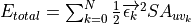
$E_{total} = \sum_{k=0}^N\frac{1}{2}\overrightarrow{\epsilon_k}^2SA_{uv_k}$

where $S$ is the stiffness tensor of the defined material and N is the total number of mesh elements.

Parameters

normalized_2d – 2D representation of a 3D model
fiberpoints – uv parameterization
vertexids – Vertex indices of each element in the 3D model
stiffness_tensor – Stiffness tensor of the given material

Returns

The computed total strain energy between normalized_2d and fiberpoints

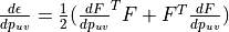
autofiber.optimization.computeglobalstrain_grad(normalized_2d, fiberpoints, vertexids, stiffness_tensor, oc)¶

Compute the gradient of the strain energy function defined above with respect to the movement of each point in the uv parameterization.

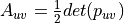
$p_{3D}$ - 2D mapping of 3D model surface based on element normal and inplanemat

$p_{UV}$ - Parameterization of 3D surface based on geodesic lines

Compute the areas of each triangular element in UV space:

$A_{uv} = \frac{1}{2}det(p_{uv})$

In order to calculate the derivative of the area of each element with respect to each nodal displacement we will calculate the (i,j)-minor of $A_{uv}$ by the determinate of the matrix created by removing the ith row and jth column in $p_{uv}$ for each element in $p_{uv}$ :

$M_{ij} = det(minor(p_{uv_{ij}}))$

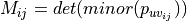
Then using $M_{ij}$ we can compute the cofactor matrix:

$Cof = ((-1)^{i+j}M_{ij})_{1 \leq i,j \leq n^*}$

Therefore, the adjugate matrix of $A_{uv}$ is:

$adj(A_{uv}) = Cof^T$

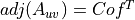
The derivative of the area of each element with respect to each nodal displacement can be calculated using Jacobi’s formula as follows:

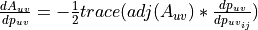
$\frac{dA_{uv}}{dp_{uv}} = -\frac{1}{2}trace(adj(A_{uv})*\frac{dp_{uv}}{dp_{uv_{ij}}})$

where $\frac{dp_{uv}}{dp_{uv_{ij}}}$ is the derivative of each nodal displacement with respect to moving all the other nodes for each mesh element.

Compute the deformation gradient between each element in UV space and the corresponding element in 2D space:

$F = p_{3D} * p_{UV}^{-1}$

Utilizing the Lagrangian finite strain tensor:

$\epsilon = \frac{1}{2}(C - I)$

where $C = F^{t}F$ the right Cauchy–Green deformation tensor and $I$ is the identity matrix.

Since $\overrightarrow{\epsilon} = [\epsilon_{11}, \epsilon_{22}, \gamma_{12}/2]$ we have to:

$\overrightarrow{\epsilon} = \frac{\epsilon}{[1.0, 1.0, 0.5]}^T$

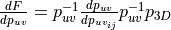
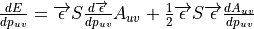
The derivative of the deformation tensor with respect to each nodal displacement is as follows:

$\frac{dF}{dp_{uv}} = p_{uv}^{-1}\frac{dp_{uv}}{dp_{uv_{ij}}}p_{uv}^{-1}p_{3D}$

The derivative of strain with respect to each nodal displacement:

$\frac{d\epsilon}{dp_{uv}} = \frac{1}{2}(\frac{dF}{dp_{uv}}^TF + F^T\frac{dF}{dp_{uv}})$

Then to account for $2\gamma_{12}$ :

$\frac{d\overrightarrow{\epsilon}}{dp_{uv}} = \frac{\frac{d\epsilon}{dp_{uv}}}{[1.0, 1.0, 0.5]}$

Finally, we can compute the derivative of the strain energy density with respect to each nodal displacement with the following application of the chain rule:

$\frac{dE}{dp_{uv}} = \overrightarrow{\epsilon}S\frac{d\overrightarrow{\epsilon}}{dp_{uv}}A_{uv} + \frac{1}{2}\overrightarrow{\epsilon}S\overrightarrow{\epsilon}\frac{dA_{uv}}{dp_{uv}}$

Parameters

normalized_2d – 2D representation of a 3D model
fiberpoints – uv parameterization
vertexids – Vertex indices of each element in the 3D model
stiffness_tensor – Stiffness tensor of the given material
oc – A vertex index which we want to constrain by fixing it’s location

Returns

The gradient of strain energy with respect to movement of each point in the uv parameterization

autofiber.optimization.minor(arr, i, j)¶

https://stackoverflow.com/questions/3858213/numpy-routine-for-computing-matrix-minors Calculate the minor of a matrix with ith row, jth column removed

Parameters

arr – Matrix of interest
i – row to remove
j – column to remove

Returns

minor of arr with ith row removed and jth column removed

AutoFiber analyze_uv¶

autofiber.analyze_uv.BuildEdgeDict(surface)¶

Create edge dictionary from a surface. The edge dictionary is indexed by a tuple (vertexindex1,vertexindex2) of indices into surface.vertexes. It contains a list of polygon ids that have an edge that shares these two vertices.

This function assumes that identical vertices in the surface have been merged, so the vertexindex uniquely identifies the vertex.

This function returns the edge dictionary

autofiber.analyze_uv.DetermineAdjacency(surface, edges, surfaceparameterization=None, texture=False)¶

Build an adjacency index for the given surface: with the given edgedict. The adjacency index has the same layout as surface.vertexidx, but additional entries may be -1 as facets may have fewer adjacencies than vertices.

The adjacency index contains the polygon numbers adjacent to the given polygon.

If texture=True is given as a parameter, then the adjacency index built up will only show adjacencies both in the polygon mesh and in the texture. In that case, the polygon indices will include both original polygons and redundant copies, so the polygon indices will range from 0 to vertexidx_indices.shape[0]+texcoordredundant_polystartindexs.shape[0]

autofiber.analyze_uv.FindTexPatches(surface, texadjacencyidx, surfaceparameterization=None)¶: Given a surface and a texture adjacency index (which contains the texture polygon numbers adjacent, to the given texture polygon, with polygons findable from surface.vertexidx_indices and surfaceparameterization.texcoordredundant…), separate the polygons of the surface into groups that have adjacent texture. Return a list of lists of polygon numbers.

autofiber.analyze_uv.IdentifyTexMaps(part, surfaceparameterizationmapping=None)¶

Trace through and identify all texture maps, given a part (ndepart instance)

If texture_urls are given through an appearance node, those are used. If the appearance node is missing or does not provide a texture_url, then a numbered name is used for that surface, of the form _unnamed_surface_%d

Returns a tuple of two dictionaries:: surface_texurl is indexed by the id of the surface object and contains the the texture url as a string. surfaces_bytexurl is indexed by texture url strings and contains a list of surface objects that share that texture url

Submodules¶

AutoFiber generator¶

AutoFiber geodesic¶

AutoFiber optimization¶

AutoFiber analyze_uv¶

AutoFiber

Navigation

Related Topics